Understanding the LLM Twin Concept and Architecture

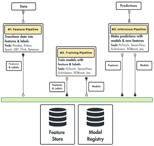
Building ML systems with feature/training/inference pipelines

The problem with building ML systems

Feature pipeline: takes raw data as input, processes it, and outputs features and labels. It stores the results in a feature store, which keeps the outputs and tracks their versions.
Because the features are versioned, we can keep the training-time and inference-time features aligned.

Training pipeline: takes features and labels and outputs a trained model. The model is stored in a model registry.
The model registry stores, versions, tracks, and shares models with the inference pipeline.
Most modern model registries also include a metadata store that lets you track essential details about how the model was trained (which features, label sets, versions, etc.).

Inference pipeline: Takes the features from the feature store and the trained model from the model registry and uses them to make predictions (either batch or real-time).

There can be more pipelines than this. For example, you can split the feature pipeline into one that computes and one that validates, or the training into training and evaluation.

RAG Feature Pipeline

An overview of advanced RAG

The traditional, vanilla RAG design can be optimized at:

Pre-retrieval: usually by pre-processing the data for indexing or query optimization
Retrieval: usually by using better embedding models, using metadata filtering
Post-retrieval: usually by filtering out noise from the retrieved documents and compressing the prompt before sending to an LLM

Note here that the aim of this chapter was to improve the vanilla RAG design. Otherwise I’d be suggesting a bunch of other stuff here.

Pre-retrieval

When optimizing this step, we might optimize at either the data indexing or query optimization stages.

In the data indexing stage, we could:

Keep a sliding window to introduce overlap between text chunks and retain important context near chunk boundaries.
Enhance granularity by removing irrelevant details, verifying facts, and updating outdated info.
Add and use metadata (tags, dates, URLs, external IDs, chapter markers, etc.).
Optimize index structures (e.g. chunk size, using multi-indexing strategies).
Store an embedded version of a smaller chunk during retrieval but then return a larger piece of context if it hits (small-to-big).

For query optimization, we could:

Route based on the user’s query (query routing)
Rewrite the user’s query. There are many ways, but:
- Paraphrase the user’s query
- Substitute less common words with more common synonyms
- Sub-queries: breaking longer queries into multiple, more focused sub-queries
Hypothetical document embeddings (HyDE): Have an LLM create a hypothetical response. Use both that and the user’s query during retrieval.
Query expansion: adding terms, concepts, etc., to the user’s query, enriching it
Self-query: map unstructured queries into structured ones. E.g. filter by metadata extracted from query before querying

Retrieval

You can either improve the embedding model, or use the DB’s filter and search features, to optimize this stage.

You can try to use hkunlp/instructor-xl · Hugging Face instead of fine-tuning an embedding model. But fine-tuning is also a good option.

As for doing better search, try using hybrid search (blend of vector and keyword-based). Keyword-based is especially good when there are domain keywords to find, as embedding models aren’t always exposed to those during training.
Or, you can try filtered vector search, where you filter by metadata on specific keywords, and then do the standard vector search.

It’s common to start with filtered vector search or hybrid search before reaching for fine-tuning.

Post-retrieval

This phase is usually used to remove noise in the context and to make sure the input is within the LLMs context window.

Two popular methods:

Prompt compression, wherein you remove unnecessary details
Re-ranking, where you use a cross-encoder ML model to give a matching score between the user’s input query and every retrieved chunk. Then you sort by score and keep only the top N results.
- For cross encoders, the pipeline is usually (query, retrieved text) → BERT → classifier → score between 0 and 1.

Exploring the LLM Twin’s RAG feature pipeline architecture

Change data capture: syncing the data warehouse and feature store

CDC is a strategy that allows you to optimally keep two or more data storage types in sync, without computing and I/O overhead. CRUD operations on the source DB are captured and replicated on the target DB. You can add additional preprocessing steps.

CDC methods use either a push-based or pull-based strategy.

With the push strategy, the source DB is the primary driver - it actively identifies and transmits data modifications to target systems. This makes the data sync almost instantaneous, but can be brittle if the target systems are inaccessible - so a message queue is often used as a buffer.

And with the pull based strategy, the source DB only records data changes. Target systems pull these regularly and update their data accordingly. This introduces a delay in data propagation - and again we use a messaging system to prevent data loss.

Here are a few CDC patterns used in the industry:

Timestamp-based: Adding a modification time to DB tables (LAST_MODIFIED or LAST_UPDATED). Downstream systems can query this to find records that have been updated since they last checked. This is simple, but is limited.
Trigger-based: Uses DB triggers to automatically record data modifications in a separate table on INSERT, UPDATE, or DELETE operations. The method is comprehensive, but can impact DB performance by adding additional write operations for each event.
Log-based: Databases maintains transaction logs to record all data modifications with timestamps. These are primarily used for recovery, but can be used to propagate changes to target systems in real time. This method also reduces performance impact on the source DB, captures all changes, and doesn’t require schema modifiations. But log formats aren’t standardized, so you might need to implement it.

Supervised Fine-Tuning

Creating an instruction dataset

Data curation
- Task specific: collect or create examples.
- Domain-specific: might require collaboration with domain experts to get examples. Quality and relevance matters.
Rule-based filtering
- Examples: length filtering, keyword exclusion, format checking.
- Fast and efficient, making it scalable.
- But needs regular review, doesn’t handle nuances well, and poor rules can create or strengthen biases.
Data deduplication
- Data diversity is important. Duplicates or near-duplicates can lead to overfitting, biased performance, inefficient training, and inflated evaluation metrics.
- Methods:
  - exact deduplication (normalize → hash → remove dupes)
  - fuzzy deduplication with MinHash deduplication (or semantic similarity)
Data decontamination: ensuring the training dataset doesn’t contain samples identical or highly similar to those in the evaluation or test sets. Uses similar techniques to those in the data deduplication step.
Data quality evaluation to check for e.g. accuracy, diversity, and complexity.
- Traditionally uses human annotation, which is highly accurate but resource-intensive.
- But we increasingly use LLMs as judges, reward models, and classifiers trained for quality prediction.
- Reward models essentially take an instruction and answer pair and return a score as output. They are often created by adding a linear head on top of a decoder-only architecture (like Gemma or Llama). Then they’re trained for this purpose, either with RL or traditional fine-tuning.
Data exploration is a continuous process. Includes both manual inspection and automated analysis. You need to understand the dataset’s characteristics, strengths, and potential shortcomings.
- You might be tempted to skip the manual exploration. Don’t! It’s important. You’ll spot errors and inconsistencies that could have been missed.
- You might use e.g. Stratified Sampling to select diverse samples, systematic review using a criteria checklist, and collaborative review with multiple reviewers.
- Statistical analysis can help reveal vocabulary diversity, potential biases, and concept representations.
- Topic clustering groups similar documents or pieces of text to surface themes and patterns in the data. You could go further and find sub-clusters.
Data generation, when there isn’t sufficient data.
- Manual generation or crowdsourcing is resource-intensive.
- Synthetic data generation with LLMs is more efficient and scalable, and can produce high-quality data if done well.
- You often start the synthetic data generation process by creating a set of carefully designed prompts (sometimes called taxonomy). These are the foundation for generating new, diverse examples.
- Synthetic data generation pipelines often use multiple steps to ensure high data quality—for example, generating an initial set of questions/instructions, generating corresponding answers/responses, and adding a validation step where another model checks accuracy, relevance, and adherence to criteria.
- You can use synthetic data generation to patch gaps in existing datasets.
Data augmentation is the process of increasing both quantity and quality of data samples.
- Method: Evol-Instruct, which uses LLMs to evolve simple instructions into more qualitative ones. These instructions can then be used to generate answers using more powerful LLMs.
- Method: UltraFeedback, which focuses on answer quality rather than instruction quality. Uses AI feedback to enhance the quality and diversity of model responses.

Creating our own instruction dataset

We’ll use backtranslation and rephrasing.

Backtranslation means providing answers and generating corresponding instructions.

Essentially we just prompt an LLM to give us instruction-answer pairs. The instructions should ask to write about a specific topic (defined by the context, e.g. a chunk of an article). The answer should provide a relevant paragraph based on the context.

Exploring SFT and its techniques

When to fine-tune

Start with prompt engineering on either open-weight or closed-source models.
Your problem might very well be solved with just that, maybe with few-shot or RAG.

This also gives you the opportunity to build a robust evaluation pipeline to measure metrics like accuracy, cost, and latency.
If the results of prompt engineering don’t live up to your requirements, you should start thinking about creating an instruction dataset. If you can do that, fine-tuning is an option.

It is generally understood that SFT leverages pre-existing knowledge in the base model’s weights and refocuses the parameters for a specific purpose.

So if what you’re trying to have it learn is too far from that, it might be difficult for it to learn. And fine-tuning a model on new knowledge could even result in more frequent hallucinations.

Parameter-efficient fine-tuning techniques

Currently, there are three main ones:

Full fine-tuning: retraining every parameter in the base model.
- Often provides the best results, but is very costly.
- Estimate GPU memory requirements by summing parameters, gradients, optimizer states, and activations
  - Params: depends on data type - for FP32 it’s 4 bytes per parameter, 2 for FP16/BF16.
  - Gradients: 4 bytes per parameter
  - Optimizer states: e.g. running avg. of past gradients and past squared gradients for each param. For Adam it’s 8 bytes per parameter.
  - Activations: vary, but are usually negligible.
  - So e.g. 112 GB of VRAM for a 7B model, and 1120 GB for a 70B model.
  - But it’s often an underestimate due to e.g. additional memory needed for activations, temporary buffers, and overhead.
- Some techniques to reduce memory usage during fine-tuning:
  - Model parallelism to spread workload across multiple GPUs
  - Gradient accumulation to enable larger effective batch sizes without the proportional memory increase
  - Memory-efficient optimizers to reduce footprint of optimizer states
  - Activation checkpointing
  - Mixed precision
- Since we directly modify the pre-training weights, this approach is ‘destructive’ and can erase previous knowledge and skills (called “catastrophic forgetting”).
Low-rank Adaptation (LoRA): introduces trainable low-rank matrices that modify the behavior of the model without changing the original parameters.
- Can fine-tune a 7B model on a single GPU with as little as 14-18 GB VRAM.
- Can achieve comparable or better results than full fine-tuning.
QLoRA: combines quantization with LoRA.
- Quantizes the base model parameters to a custom 4-bit NormalFloat (NF4) data type. Like LoRA, it then introduces small, trainable low-rank matrices (adapters) to specific layers. The remaining weights are unchanged.

Fine-tuning in practice

Here’s the code I used to fine-tune a Llama model. I used a Modal notebook with a H100 GPU. The fine-tuning process fit well within the free credits you receive.

Final model: cbbh/TwinLlama-3.1-8B · Hugging Face

%uv pip install unsloth comet-ml

import os
import torch
from unsloth import FastLanguageModel, is_bfloat16_supported
from trl import SFTTrainer
from datasets import load_dataset, concatenate_datasets
from transformers import TrainingArguments, TextStreamer

HF_TOKEN="redacted"
COMET_API_KEY="redacted"

os.environ["HF_TOKEN"] = HF_TOKEN
os.environ["COMET_API_KEY"] = COMET_API_KEY

max_seq_length = 2048
model, tokenizer = FastLanguageModel.from_pretrained(
    model_name="meta-llama/Meta-Llama-3.1-8B",
    max_seq_length=max_seq_length,
    load_in_4bit=False
)

model = FastLanguageModel.get_peft_model(
    model,
    r=32,
    lora_alpha=32,
    lora_dropout=0,
    target_modules=["q_proj", "k_proj", "v_proj", "up_proj", "down_proj", "o_proj", "gate_proj"]
)

dataset_1 = load_dataset("cbbh/llmtwin", split="train[:100]")
dataset_2 = load_dataset("mlabonne/FineTome-Alpaca-100k", split="train[:10000]")
dataset = concatenate_datasets([dataset_1, dataset_2])

alpaca_template = """Below is an instruction that describes a task. Write a response that appropriately completes the request.
### Instruction:
{}
### Response:
{}
"""

EOS_TOKEN = tokenizer.eos_token

def format_samples(examples):
    text = []
    for instruction, output in zip(examples["instruction"], examples["output"], strict=False):
        message = alpaca_template.format(instruction, output) + EOS_TOKEN
        text.append(message)
    return {"text": text}

dataset = dataset.map(format_samples, batched=True, remove_columns=dataset.column_names)

dataset = dataset.train_test_split(test_size=0.05)

trainer = SFTTrainer(
    model=model,
    tokenizer=tokenizer,
    train_dataset=dataset["train"],
    eval_dataset=dataset["test"],
    dataset_text_field="text",
    max_length=max_seq_length,
    dataset_num_proc=2,
    packing=True,
    args=TrainingArguments(
        learning_rate=3e-4,
        lr_scheduler_type="linear",
        per_device_train_batch_size=2,
        gradient_accumulation_steps=8,
        num_train_epochs=3,
        fp16=not is_bfloat16_supported(),
        bf16=is_bfloat16_supported(),
        logging_steps=1,
        optim="adamw_8bit",
        weight_decay=0.01,
        warmup_steps=10,
        output_dir="output",
        report_to="comet_ml",
        seed=0
    )
)

trainer.train()

FastLanguageModel.for_inference(model)
message = alpaca_template.format("Write a paragraph about QuickAdd for Obsidian.", "")
inputs = tokenizer([message], return_tensors="pt").to("cuda")
text_streamer = TextStreamer(tokenizer)
_ = model.generate(**inputs, streamer=text_streamer, max_new_tokens=256, use_cache=True)

model.save_pretrained_merged("model", tokenizer, save_method="merged_16bit")
model.push_to_hub_merged("cbbh/TwinLlama-3.1-8B", tokenizer, save_method="merged_16bit")

Fine-Tuning with Preference Alignment

Understanding preference datasets

In preference datasets, each instruction is paired with one preferred answer and one rejected answer. The objective is to train the model to generate the preferred response rather than the rejected one.

It would essentially be an instruction set if not for the rejected answer.

Using preference alignment can be more beneficial than just SFT alone in contexts like chatbots, content moderation, summarization, code generation, creative writing, and translation.
It helps capture subjective factors - the hard-to-capture subtleties of what makes a response better than another. The nuances.
What people prefer over mere instruction-following and correctness.

Usually requires fewer samples than instruction datasets.

General-purpose alignment: millions of samples.
Small-scale: 10k to 100k samples to enhance model performance. Both to improve benchmark scores and to heal networks after merging, pruning, and other modifications.
Specific tasks (like the ones mentioned above) require fewer samples. Like 100 to 10,000. E.g. you can train a model to claim it was trained by you with ~200-500 pairs.

DPO is generally less destructive and milder on the model than SFT.

Data generation and evaluation

There are generally 4 categories of methods to create and evaluate DPO datasets:

Human-generated, human-evaluated datasets: hire people to both create responses to prompts and to evaluate them. Ideal for complex tasks, but very resource intensive.
Human-generated, LLM-evaluated datasets: useful if you already have lots of human-generated data, but rarely used in practice due to inefficiency.
LLM-generated, human-evaluated datasets: offers a good balance between quality and efficiency. Have the LLM generate multiple responses and humans rate them.
LLM-generated, LLM-evaluated datasets: fully synthetic is becoming increasingly common because of the scalability and cost-effectiveness. Requires careful prompting to ensure quality and diversity.

When writing prompts for synthetic generation, it’s generally good to aim for varied outputs. E.g. when creating a summarization dataset, ask for varying lengths, details, focus, and style.

It can be better to use multiple models to generate samples.

To evaluate samples with LLMs, you need to develop detailed criteria. Your prompt should clearly communicate those guidelines to the model, so it can best select preferred and rejected responses.

LLM evaluation for preference datasets can be done through absolute scoring or pairwise ranking.

Absolute scoring: LLM assigns a numerical score or categorical rating to each response based on the criteria. Straightforward but potentially inconsistent across prompts or evaluation sessions.
- Prompt outlines the eval criteria and asks for a score (e.g. 1-5, poor/fair/good/excellent). Only judges 1 response.
Pairwise ranking: presenting the LLM with two responses and asking it to choose between the better one or rank them. Can lead to more consistent results.
- Prompt asks model to compare 2 responses, asking which is better e.g. in terms of relevance, coherence, and helpfulness.
- Can improve by providing a ground-truth answer and using chain-of-thought reasoning.

Pairwise is generally better & more accurate.

Varying the order of A/B in pairwise ranking can help reduce the effect of position bias—LLM judges tend to prefer the first answer.
Providing few-shot examples can help reduce the judge’s length bias (prefers longer answers) and family bias (prefers models from the same family).

Creating our own preference dataset

In the interest of creating an LLM Twin: preferred answers will be chosen from our text, and rejected answers generated by the model.

It takes time and iterations to get the right prompt to generate the data.
Adjust prompt → Look at the results → Repeat until happy.

Preference alignment

Reinforcement Learning from Human Feedback

Basically you use the preference dataset to train a reward model (RM) to predict a higher scalar value for the preferred answer.

You freeze a reference model (usually the SFT model) and use it as the anchor distribution you don’t want to drift too far from.

The current policy (the trainable model) samples completions for a batch of prompts.
The RM scores each completion to give a scalar reward.
That reward is almost always shaped with a KL term to the reference, meaning the reward is regularized by an additional Kullback-Leibler (KL) divergence factor. This reduces drift from the model before training (our reference model; frozen).

Proximal Policy Optimization (PPO) then optimizes the policy using the shaped reward.

Direct Preference Optimization

Since RLHF, the process has seen improvements. Direct Preference Optimization is one such modern alternative.

DPO tries to skip the explicit reward model and optimize directly on the preference pairs. This trades off some flexibility for simplicity and stability.

DPO can be implemented as a binary Cross Entropy loss function that operates directly on the language model’s output probabilities. It encourages the model to assign higher probabilities to preferred responses and lower to non-preferred ones.

Implementing DPO

The objective in creating the LLM twin is imitating a writing style. That conflicts with the natural tendency of DPO to encourage formal language. So we’ll do light fine-tuning, with a low learning rate and a small number of epochs.

Here’s the code I used. As with SFT, I ran this in Modal notebooks with a H100 GPU.

Final model: cbbh/TwinLlama-3.1-8B_dpo · Hugging Face

%uv pip install unsloth comet-ml

import os

HF_TOKEN="redacted"
COMET_API_KEY="redacted"

os.environ["HF_TOKEN"] = HF_TOKEN
os.environ["COMET_API_KEY"] = COMET_API_KEY

from unsloth import PatchDPOTrainer

PatchDPOTrainer()

import torch
from unsloth import FastLanguageModel, is_bfloat16_supported
from trl import DPOConfig, DPOTrainer
from datasets import load_dataset, concatenate_datasets
from transformers import TrainingArguments, TextStreamer

max_seq_length = 2048
model, tokenizer = FastLanguageModel.from_pretrained(
    model_name="cbbh/TwinLlama-3.1-8B",
    max_seq_length=max_seq_length,
    load_in_4bit=False
)

model = FastLanguageModel.get_peft_model(
    model,
    r=32,
    lora_alpha=32,
    lora_dropout=0,
    target_modules=["q_proj", "k_proj", "v_proj", "up_proj", "down_proj", "o_proj", "gate_proj"]
)

dataset = load_dataset("cbbh/llmtwin-dpo", split="train")

alpaca_template = """Below is an instruction that describes a task. Write a response that appropriately completes the request.
### Instruction:
{}
### Response:
"""

EOS_TOKEN = tokenizer.eos_token

def format_samples(example):
    example["prompt"] = alpaca_template.format(example["prompt"])
    example["chosen"] = example["chosen"] + EOS_TOKEN
    example["rejected"] = example["rejected"] + EOS_TOKEN
    return {"prompt": example["prompt"], "chosen": example["chosen"], "rejected": example["rejected"]}

dataset = dataset.map(format_samples)
dataset = dataset.train_test_split(test_size=0.05)

trainer = DPOTrainer(
    model=model,
    ref_model=None,
    tokenizer=tokenizer,
    beta=0.5,
    train_dataset=dataset["train"],
    eval_dataset=dataset["test"],
    max_length=max_seq_length//2,
    max_prompt_length=max_seq_length//2,
    args=DPOConfig(
        learning_rate=2e-6,
        lr_scheduler_type="linear",
        per_device_train_batch_size=2,
        per_device_eval_batch_size=2,
        gradient_accumulation_steps=8,
        num_train_epochs=1,
        fp16=not is_bfloat16_supported(),
        bf16=is_bfloat16_supported(),
        optim="adamw_8bit",
        weight_decay=0.01,
        warmup_steps=10,
        output_dir="output",
        report_to="comet_ml",
        eval_strategy="steps",
        eval_steps=0.2,
        logging_steps=1,
        seed=0,
        dataset_num_proc=8
    )
)

trainer.train()

FastLanguageModel.for_inference(model)
message = alpaca_template.format("Write a paragraph about QuickAdd for Obsidian.", "")
inputs = tokenizer([message], return_tensors="pt").to("cuda")
text_streamer = TextStreamer(tokenizer)
_ = model.generate(**inputs, streamer=text_streamer, max_new_tokens=256, use_cache=True)

model.save_pretrained_merged("model", tokenizer, save_method="merged_16bit")
model.push_to_hub_merged("cbbh/TwinLlama-3.1-8B_dpo", tokenizer, save_method="merged_16bit")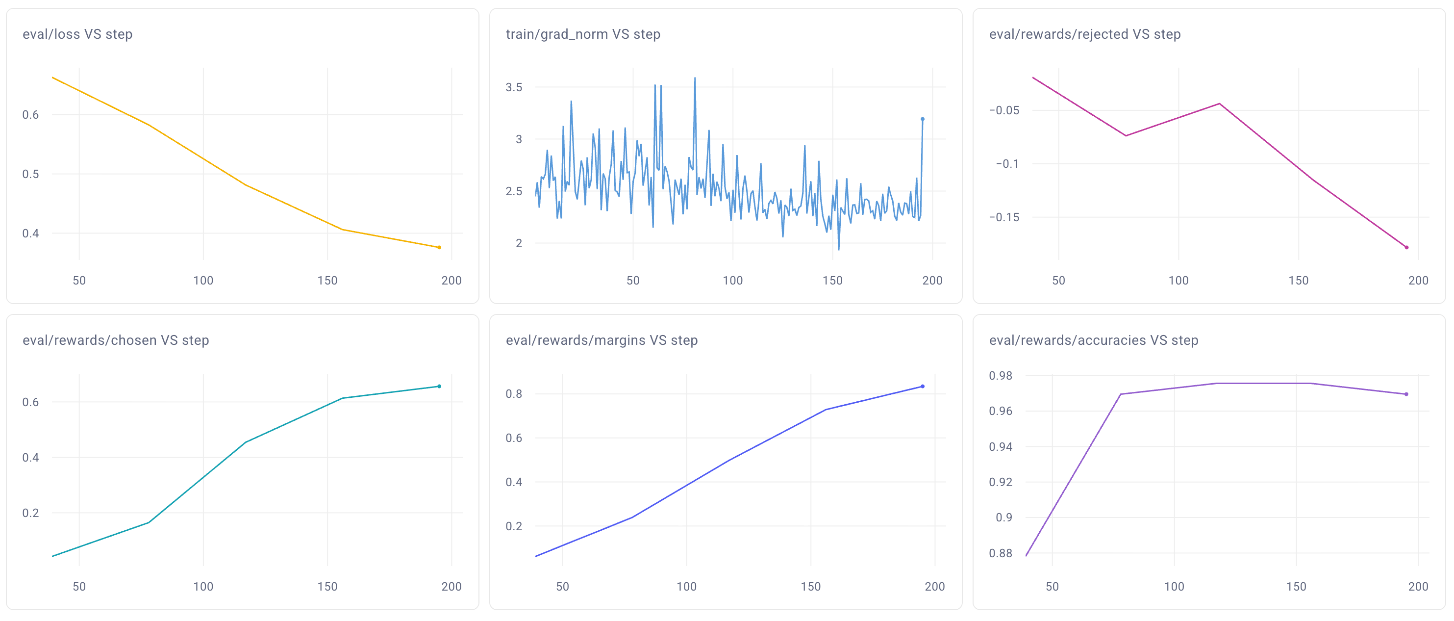

Metrics review:

Loss should continuously decrease on average.
Expect the gradient norm to stay small with only occasional spikes.
Rewards: we track chosen and rejected values corresponding to the mean difference between the log probabilities output by the trained and reference models. The model should, over time, choose the chosen answers and reject the rejected answers. The difference is tracked by the margin metric (difference between chosen and rejected rewards).
Accuracies: the percentage of times the model correctly identifies the chosen answers. Should gradually increase. Doesn’t need to reach 100% (if it does so quickly, the preference dataset is too easy; add challenging examples).

So the metrics achieved in the training run seem to be fine.

Inference Optimization

A few commonly used optimization strategies to speed up inference and reduce VRAM usage:

Static KV Cache
Continuous Batching
Speculative Decoding
Optimized Attention mechanisms

Since the KV Cache grows with each generation step and is dynamic, you can’t use torch.compile. Using a static KV cache solves that by pre-allocating the KV Cache size to a maximum value, so you can use torch.compile. This can lead to a 4x speedup.

Before we dive in, here are some inference engines you can use for your projects:

Continuous Batching

Traditional batching: wait for the longest request to finish before starting a new batch.
→ The accelerator will sit partly idle, waiting for a straggling request to finish → under-utilization.

Continuous batching (in-flight batching): immediately feed a new request into the batch as soon as one completes to prevent idle time.
Sometimes you need to pause the generation process to run prefill, or to embed and encode waiting requests. So balancing generation and prefill means tuning the wait-to-serve ratio.

Speculative decoding

Also called assisted generation.

Even with continuous batching, we don’t use the full parallel processing capabilities of the accelerator.
Speculative decoding uses the spare compute to predict multiple tokens simultaneously, using a smaller proxy model.

Generally:

Use a smaller model (like distilled or pruned from the main) to predict multiple tokens in parallel (5-10 maybe)
Feed these into the full model to validate which predictions match what it would have generated
Retain the longest matching prefix and discard any incorrect tokens

If the small model is good at approximating the large model, you can generate multiple tokens in a single step.

You have a fast draft model and a larger target model .
The goal is to generate from , but cheaply, by letting propose several tokens and having verify them in one pass.

→ I decided to just read the paper: Fast Inference from Transformers via Speculative Decoding .

Data parallelism

This is a simple type of model parallelism.

Make copies of the model and distribute them across different GPUs.
Each GPU processes a subset of the data simultaneously.

During training, average the gradients computed on each GPU and use the average to update the model parameters.

During inference, it can process concurrent requests.

Limited by model size (must fit on a single GPU) and communication overhead between GPUs.
DP is mostly used for training. Pipeline and tensor parallelism are preferred for inference.

Pipeline parallelism

Introduced in the GPipe paper (2019).
It’s a strategy for distributing the computational load of training and inference across multiple GPUs.

Instead of replicating the entire model on each GPU (like in data parallelism), this partitions the model’s layers across GPUs.

During the forward pass, activations are computed and passed along to the next GPU.
For training, the backward pass follows a similar sequence in reverse: gradients are propagated back through the GPUs.

The number of GPUs is often referred to as the degree of parallelism.

Tensor parallelism

Another popular technique distributes the computation of LLM layers across multiple devices. This approach splits the weight matrices within individual layers.

Model quantization

Weights are typically stored in FP16 or FP32 by default. This means higher precision but at the cost of increased memory usage and computational complexity. We can use quantization to reduce memory footprint and speed up inference.

Two main approaches to weight quantization:

Post-Training Quantization (PTQ): convert weights of a pre-trained model to a lower-precision format without retraining. Can cause performance degradation.
Quantization-Aware Training (QAT): do quantization during training or fine-tuning, allowing the model to adapt to the lower precision weights. Often gives better results than PTQ.

Data type matters here. Floating-point numbers are often represented by FP32, FP16 (called half-precision), or BF16 (brain floating-point) in deep learning settings.
These formats allocate a fixed number of bits to represent the sign, exponent, and significand (mantissa) of a number.
All use 1 bit for the sign, but then:

FP32: 8 bits for the exponent, 23 bits for the significand
FP16: 5 bits for the exponent, 10 bits for the significand
BF16: 8 bits for the exponent, 7 bits for the significand

A sign of indicates a positive number, and a negative.
The exponent controls the range that is represented (big or small), and the significand controls the precision of the number (number of digits).

To convert the representations to real numbers:

Representing in each:

FP32:
FP16:
BF16:

Neural Networks seem to prefer a bigger range over better precision, which is why BF16 is the most popular data type, when the hardware supports it.

You don’t have to quantize to the above data types. There are many others, like INT8.

E.g. you can use absolute maximum (absmax) quantization or zero-point quantization to quantize any of the above three into INT8.

Absmax quantization maps the original weights to the range by dividing them by the absolute maximum value of and scaling the :

You can dequantize with:

Note on range: Int8’s range is , but many use for symmetry, like we do above. With the symmetric choice, zero maps to code 0 exactly, which is nice and clean for signed weights.

Zero-point quantization considers asymmetric input distributions and maps the weights to the range by introducing a zero-point offset:

where and .

You can dequantize with:

These naive quantization methods are limited, especially when dealing with outliers. Discarding the outliers is not feasible (would degrade model performance).
Instead, we use more advanced quantization methods.

A few quantization techniques:

GGUF (llama.cpp’s own quantization format)
GPTQ
EXL2
Activation-aware Weight Quantization (AWQ)
Quantization with Incoherence Processing (QuIP#)
Half-Quadratic Quantization (HQQ)

RAG Inference Pipeline

receive user query
pre-retrieval optimizations (query expansion + self-querying)
filtered vector searches
collect & deduplicate
rerank
take top-K chunks
build prompt (query + context)
call SageMaker endpoint
return answer

At the end of this chapter, they recommend something I’d highlight: hybrid search.
The RAG pipeline above uses dense vector similarity search across multiple indices. It would make sense to introduce keyword search via e.g. BM25, and include those results during the reranking process. This would potentially improve the retrieval quality because this system likely would benefit from search using exact terms.

Query expansion

We do query expansion (a.k.a multi-query) because a single embedded query covers only a tiny patch of the embedding space, meaning semantically relevant items that sit in other neighborhoods may get missed.
So we use an LLM to generate N additional phrasings of the original question, embed each and run xN searches. This broadens semantic coverage at the cost of more searches, but latency can be kept down via parallelism.

The prompt for query expansion just asks the LLM to generate N different versions because it’ll help overcome some limitations of distance-based similarity search. Then it asks to separate these alternative questions by a given separator. And we pass the original question, of course.

In my experience, this is a somewhat brittle and suboptimal approach, so I would not recommend it as “best practices.”

Also: query expansion is a solution to a problem, and they aren’t really explaining that problem, and instead just jumping to a solution.
The problem is really “are we finding enough relevant documents for our answers to be good?”, or, in other words, the system sees recall-starved queries.
Query expansion is a specific tool to help with that. There are many other approaches. And other metrics (like precision) to balance, to ensure good answers.
Don’t make query expansion your default hammer to this kind of problem. Be scientific about it: create hypotheses, experiment, measure, validate, and repeat!

Self-querying

Here we extract metadata for filtering: you can’t rely on embeddings to preserve every constraint (e.g., author, tags). Even if the text mentions an author, the embedding may not weight it strongly.
So we use an LLM to extract explicit metadata (here: author_full_name or id) from the user query and store it in the Query object. Then pass them as structured filters into the vector search.

The prompt here just asks the LLM to extract either a user name or ID, or none if there is none present. Then it gives three examples (few-shot).

For example, “My user id is 1345256 and I want to write a post about…” should lead to extracting ID 1345256.

Again here I’d say the example is not ideal. The user would never write “my name is” and then their query. When you build solutions, you handle this outside the user’s query, e.g. passing it from the user’s current view on the frontend, their current session, or something else. Avoid relying on specific inputs being present, because they won’t be.
Self-querying would be super useful if the user wrote specific tags, which could be extracted. E.g. they ask “I want to write a post about RAG”, and then it extracts RAG and maybe some other tags, and finds examples of how the author writes about RAG, so that can be used for further generation.

Real systems already know who the user is and how to treat them, based on e.g. session, token, org, roles, locale, and feature flags.
Identity, tenants, and ACLs are hard filters. Do not ever outsource them to an LLM.

Inference Pipeline Deployment

There are essentially four aspects that limit you:

Latency: network + (de)serialization + LLM inference.
Throughput: requests/sec your system sustains. Often improved with dynamic batching, which can raise single-request latency but increase system-wide throughput.
Data shape and size: text vs. images, prompt/context assembly, retrieval hops, etc. adds network time.
Infrastructure: choosing the right CPU/GPU size, fast disks, and network. Over-optimizing for latency can underutilize hardware and bloat cost per request.

And there are two critical decisions that drive everything:

How synchronous is the interaction?
- Online real-time (sync): for systems with humans in the loop, like chatbots, assistants, or autocomplete. You optimize for low latency and token streaming. Cost fluctuates with traffic.
- Asynchronous (queued): for jobs that can wait (e.g. summarizing docs, transcoding video, long LLM tools). You optimize for cost and throughput, and you absorb spikes with a queue.
- Offline batch (scheduled): periodic, large-scale scoring where freshness can lag (e.g. overnight recommender system refreshes, analytics). You optimize for unit cost and development simplicity.
How decomposed is the service?
- Monolith: one deployable that does preprocessing + model + post-processing. This is the fastest to ship, and is fine for CPU-only or small models. It’s harder to scale efficiently once GPUs enter the picture.
- Microservices: at least split LLM service (which is GPU-bound) from business/RAG logic (CPU/IO-bound). This lets you scale independently, pick the right runtimes, and GPUs working.

Taking a deeper look at how to build each of the service types:

Online real-time
- Transport: REST for simplicity, gRPC for speed, WebSockets/SSE for token streaming.
- Use for: chat, interactive tools, embedding/rerank APIs in live paths.
- Needs: autoscaling, load balancing, good cold-start behavior, streaming.
Asynchronous
- Pattern: client POSTs → job queued → worker(s) process → result stored/notified.
- Use for: multi-minute jobs, bursty loads, cost control.
- Needs: durable queue, idempotency, retries, status polling or push notifications.
Offline batch
- Pattern: pull a big dataset, score in bulk, write back to storage/warehouse.
- Use for: periodic recsys, analytics, backfills.
- Needs: scheduler, big I/O, checkpointing. Accepts prediction staleness.

Since the goal in this book is building a chatbot to assist with content-creation, aiming for real-time + microservices is what we’re going with.

Business microservice in FastAPI to handle requests, retrieval, prompt assembly, calling the LLM service, and streaming the result.
LLM microservice using SageMaker and Hugging Face TGI, with a dedicated GPU instance to host the model.
Our model registry is Hugging Face Hub
Qdrant will be the online vector DB for low-latency retrieval

MLOps and LLMOps

LLMOps comes from the rise in popularity of LLMs, and builds on MLOps, which, in turn, builds on DevOps.

LLMOps concerns itself with problems specific to LLMs, like prompt monitoring and versioning, input and output guardrails, and feedback loops to gather fine-tune data. As well as training models on huge clusters, large-scale collection of tokens to use for training, and reducing infra costs.
The latter problems are usually solved by the large companies like OpenAI, Meta, and so on, so smaller companies can focus on the former set of problems.

The idea in this chapter is to leverage the principles from LLMOps, MLOps, and DevOps.
Build a continuous integration (CI) and continuous deployment (CD) pipeline to test the integrity of the code, and automate the deployment process.
Then a continuous training (CT) pipeline to automate training.
And finally, a monitoring pipeline to track all prompts and generated answers.

DevOps was born to automate the process of shipping software at scale. It’s used when you want to automate building, testing, deploying, and monitoring components.

These are the essential practices in DevOps:

Deployment Environments: Dev → Staging → Production (test before shipping)
Version Control: Track every code change (GitHub, GitLab)
Continuous Integration (CI): Automatically build and test changes
Continuous Delivery (CD): Automate infrastructure provisioning and deployment

MLOps was introduced because ML systems face unique challenges traditional software systems do not.

Data dependency: Models need continuous retraining as data changes
Model versioning: Track both code AND model weights
Feature engineering: Manage data transformations and feature stores
Model monitoring: Detect distribution drift and performance degradation

You usually go through three levels:

Level 0 (Manual): Everything done by hand, no automation
Level 1 (Automated Training): Continuous training pipeline
Level 2 (Automated CI/CD/CT): Full automation including testing and deployment

MLOps has these core components:

Model Registry: Version and share trained models
Feature Store: Centralize feature engineering logic
Orchestrator: Coordinate pipeline execution (e.g., ZenML, Airflow)
Artifact Store: Store intermediate pipeline outputs
Monitoring System: Track model performance post-deployment

Experiment tracking is a very important part of MLOps. Training ML models is an iterative and experimental process, so it’s important to be able to compare and track your experiments.

LLMOps has some key differences from MLOps. We got into one earlier: most companies won’t train from scratch.
Training foundational LLMs requires massive GPU clusters and trillions of tokens, so instead, users focus on prompt engineering, fine-tuning, and RAG.

Secondly, there are challenges specific to LLMOps:

Prompt Monitoring & Versioning: Track what prompts work and fail
Input/Output Guardrails: Prevent toxic or inappropriate content
Human-in-the-Loop Feedback: Gather data for continuous improvement
Cost Management: LLM inference is expensive; optimize token usage

While monitoring in MLOps might track accuracy, precision, and recall, in LLMOps, it’d track things like prompt quality, toxicity, or relevance.

The LLMOps stack used in this project is:

ZenML for pipeline orchestration
AWS for cloud infra (SageMaker, ECR, S3)
MongoDB and Qdrant for data storage and vector database
Opik (by Comet ML) for monitoring and observability
GitHub Actions for CI/CD automation

What to monitor in LLM systems

1. Prompt-Level Metrics:

Latency per request
Token usage (input/output)
Cost per query
User feedback scores

2. System-Level Metrics:

Request volume
Error rates
Model version performance
Infrastructure resource usage

3. Quality Metrics:

Relevance of generated responses
Toxicity detection
Hallucination detection
User satisfaction scores

And when implementing monitoring, you should also aim for:

Trace Tracking: Full request lifecycle from input to output
Span Analysis: Break down latency by component (retrieval, generation, etc.)
Feedback Collection: Thumbs up/down, ratings, comments
Dataset Creation: Automatically log prompts and responses for fine-tuning

This can be achieved with e.g. Opik, Langfuse, and similar services.

Notes on

LLM Engineer's Handbook

by Paul Iusztin & Maxime Labonne